Understanding Neural Network in Machine Learning

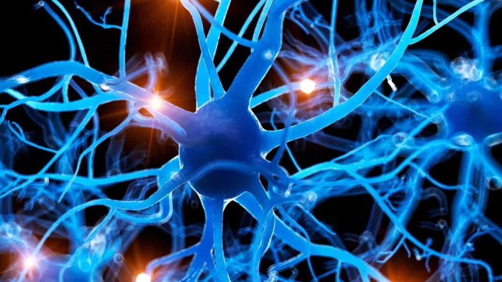
The evolving technology is highly dependent on the simplification of task today. Many aids and tools are defined to reduce human effort and intervention. Image processing is one of the emerging topics in the current era. Other than its use in medical industry, it has been playing a vital role in other fields of deep analysis and search which are popular in navigation, telecommunication, education and what not. However, image processing has brought in lime light the wonders of neural networks, whether be it artificial or conventional.

Neural network is an algorithm which makes it way in classification and image analysis tasks. Machine learning remains incomplete without the implementation of neural networks due to its excellent capacity in subsequent data analysis techniques, most preferably, Natural Language Processing. In this every data scientist’s go to classification algorithm as it requires much less processing and can perform better while training data.

ARCHITECTURE:

The framework of neural networks is much tideous to observe and understand. The architecture of neural networks works in layers. Commonly, a neural network consists of an input layer, an output layer and multiple hidden layers. The hidden layers are not literally hidden but its implementation is kept abstract from the user. It may include convolution layers, ReLU layers, pooling layers, fully connected layers, and normalization layers. 

CONVOLUTION LAYER:

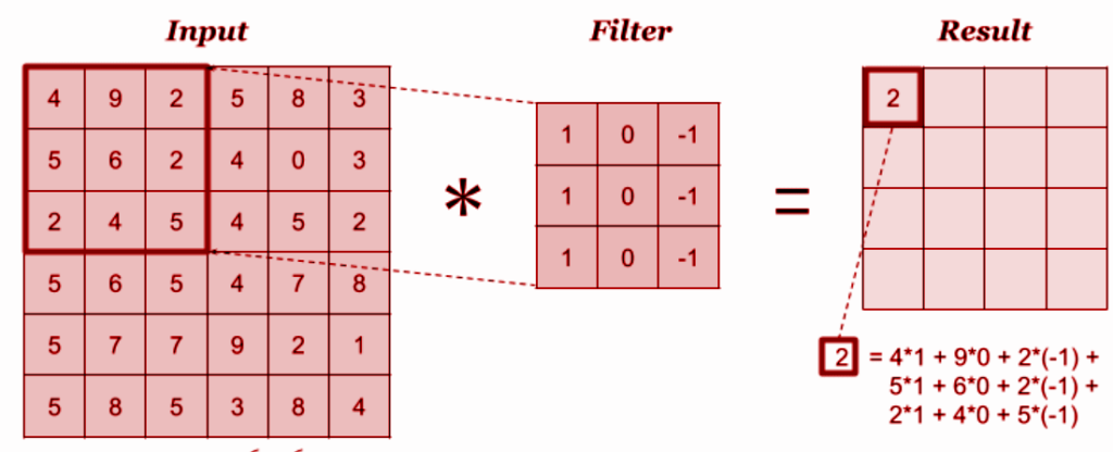
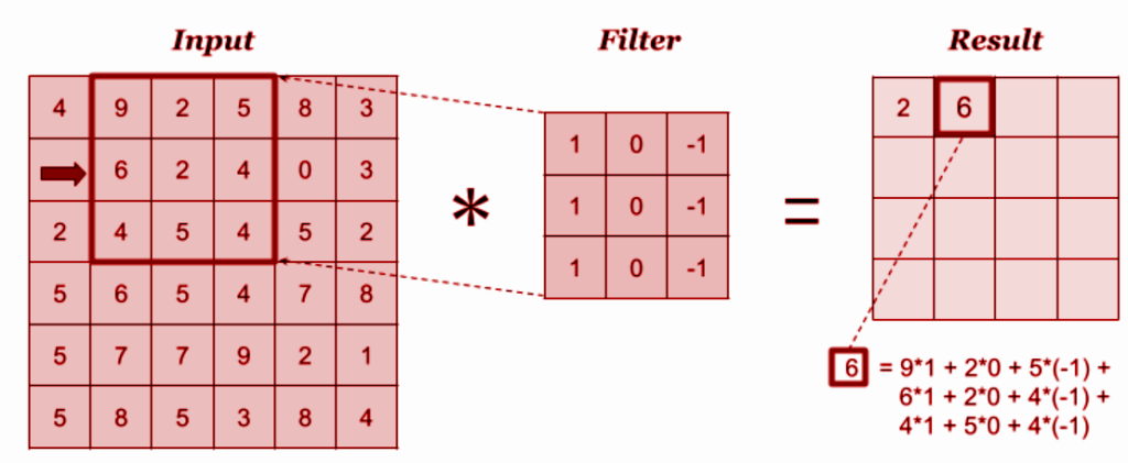
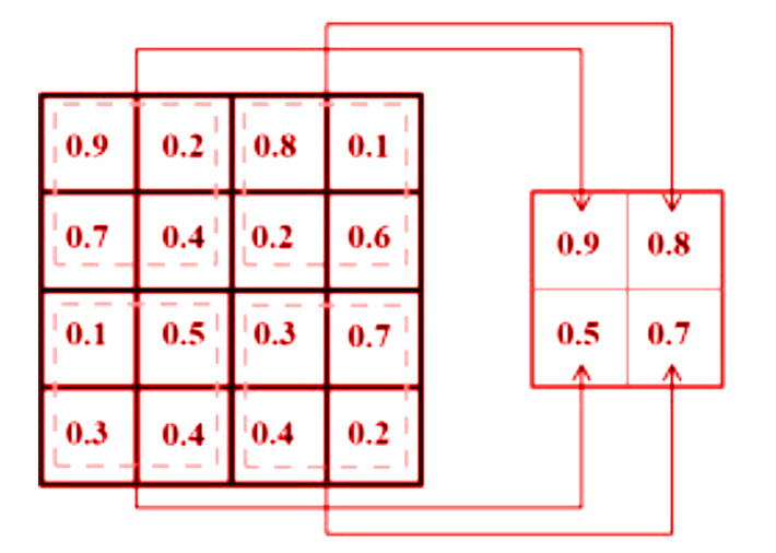
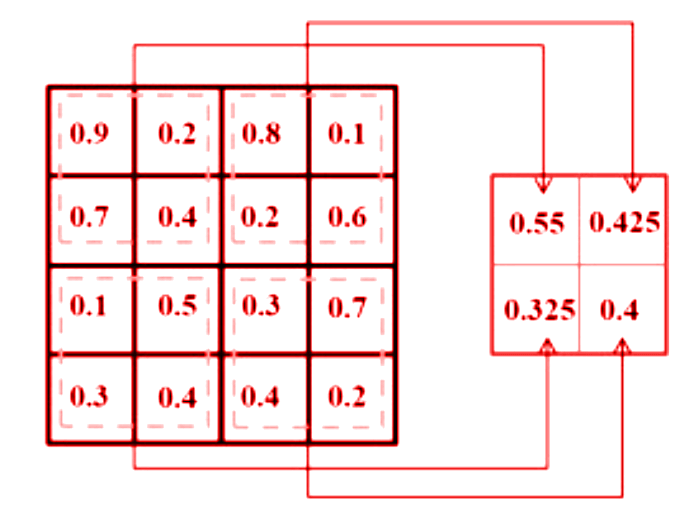
The convolution layer is the layer where one can perform mix and match or experiment with elements in the image. It uses filters to obtain different features of the image that makes sense so that meaningful results and observations can be drawn out from it.

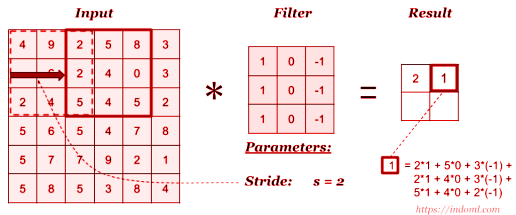
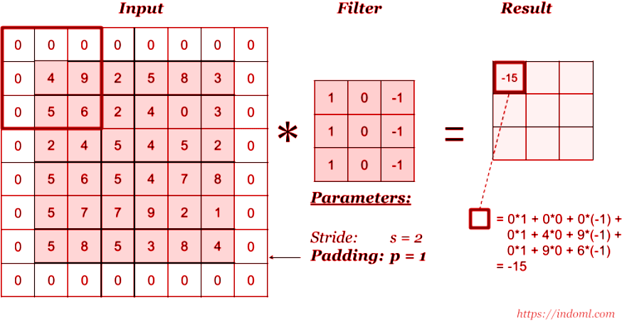
The principle rule of working with convolution layers is figuring out which filters to be applied. Filters are nothing but matrices designed in such a way that a particular output is achieved.

A given image is first passed through numerous filters coded as per requirement. The outcome includes kernel which are distinct in feature maps. Filtering works by overlaying the filter on the input section, the filters are element-wise multiplied and elements are added.

Next, we move the filter right or left according to the task and perform the same calculation to get the next result. This process is continued for the whole input till the desired output is obtained.

To precisely understand the functioning of convolution layer, lets take a look at the example below. The below image is used for testing and filters will be applied to it.

Figure before applying filters

We have 2 set of filters chosen for the demonstration:

                        Filter 1                           Filter 2

                   [ [ 1,  0, -1 ] ,                   [  [ 1,  2,  1 ] ,

                     [ 2,  0, -2 ] ,                      [ 0,  0,  0 ] ,

                     [ 1,  0, -1 ]  ]                     [-1, -2, -1 ]  ]

Image after applying filter 1
Image after applying filter 2

The convolution layer further has two operations – stride and padding

Stride: It determines the number of pixels to be shifted over input matrix. For instance, when the stride is 2, the filter moves 2 pixels at a time.

Padding: Convolution can make the image shrink and if there a numerous filters the image still has to pass, it is possible that information and performance of the image will degrade. This is when padding comes to rescue. It deals with this vanishing problem by allowing us to use the convolution layer without necessarily shrinking the width and the height of the image.

The neural networks have two main operations, namely, convolution operation and pooling operation. As from the above example one might have understood that convolution operation uses filter to extract feature maps from the datasets to preserve important spatial details.

Pooling operation, otherwise known as sub-sampling operation, is a technique where the dimensionality of the feature map can be reduced from the convolution operation using max pooling and average methods.

The framework description can be concluded by stating that neural networks have minimal resemblance with the standard architecture. There is no convention that each node or neuron in the circuit should be connected to the previous neuron in the previous layer. But some nodes are connected in a special region known as the local receptive field.

POOLING LAYER:

The pooling layer is used immediately after the convolution layer. This layer maintains the information simplified and reduces the scale feature of maps. It works by making a condensed feature map from each feature map in the convolution layer. Pooling operation can be performed in various types such as geometric average, harmonic average and maximum pooling as they efficiently reduce the computational time and over-fitting issues.

Maximum Pooling
Average Pooling
FULLY CONNECTED LAYERS:

Placed after convolution and pooling layers, the fully connected layers form the final layers in the neural network structure. The goal is to comprise the entire composite and aggregates the most important information from all the neural networks procedures. This layer is responsible for providing a feature vector for the input data so as to perform prediction and classification. Softmax layer, the last layer of fully connected layer, determines the probability of input image belonging to each target class.

APPLICATIONS:

While developing neural networks based application, one needs to tune many hyper parameter with care as they have a significant effect on the CNN structure such as depth, number of strides, and pooling capacity, which makes it a challenging task. Finding the appropriate hyper parameters is performed as a trail and error process and requires experience.

The two most commonly used methods are – from scratch training and transfer learning.

From scratch:

In this method, you need to start from zero. The tasks included are figuring the number of layers, designing filters and acquire massive amount of data if the network is deep. This is obviously time consuming and has a very high computation cost due its resources while keeping in mind that only the correct data gets labelled.

Transfer learning:

Transfer learning is a faster and an easier way to inculcate deep learning. Here, pre-trained models are used to target application. Pre-trained models have the ability to learn the complex function which helps to train the new targets, avoid the burden of training from scratch. One can also manipulate the framework by freezing some pre-trained layers and adding new layers as per the user’s need.

Leave a Reply

Your email address will not be published. Required fields are marked *